The SQL Tab: Reading Physical Execution Plans
The SQL Tab is where DataFrame and Spark SQL code stops being an abstraction and becomes a concrete, inspectable execution plan. Every time you call an Action on a DataFrame (as opposed to a raw RDD), Spark's Catalyst Optimizer compiles it into a Physical Plan, and this tab renders that plan as an interactive graph with live metrics on every node.
The tab's landing page lists every query that's run, each linking to its own plan:
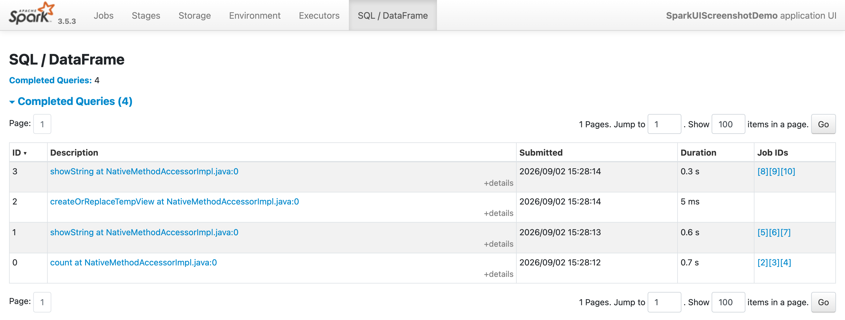 Figure 1 — SQL Tab: every DataFrame/SQL query executed, with duration and Job IDs.
Click into one and you get the full physical plan graph:
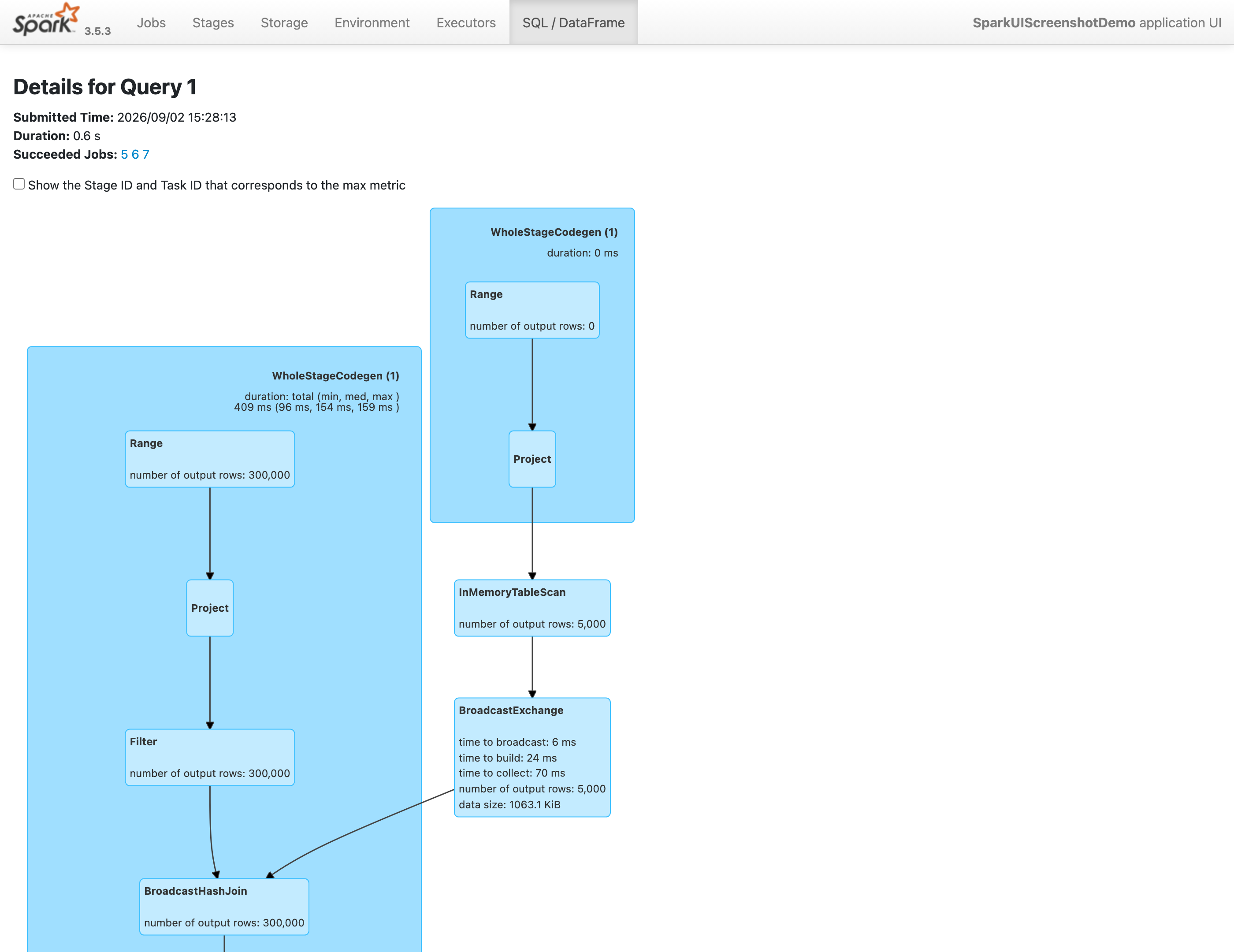 Figure 2 — SQL Query DAG: the physical plan for a broadcast join, with row counts on every operator.
Reading the Physical Plan Graph
Each box in the graph is a physical operator. The most common ones you'll see, in roughly the order data flows through them:
FileScan/Scan parquet/Scan csv: The read from source. Look at its metrics —number of files readandsize of files readtell you whether partition pruning and predicate pushdown actually worked (i.e. Spark only read the files your filter needed, not the whole table).Filter: AWHEREclause. If this appears after a largeScaninstead of being pushed into it, you're paying to read and deserialize rows you're about to throw away.Project: A column selection (SELECT col1, col2). Cheap, but worth confirming it's dropping columns you don't need before an expensive shuffle, not after.Exchange: A shuffle. This is the single most expensive operator type — it means data is being repartitioned across the network. EveryExchangenode has a "shuffle records written" metric worth checking against your expected row count.BroadcastExchange→BroadcastHashJoin: The fast join path — one side of the join is small enough to be shipped whole to every executor, avoiding a shuffle of the large side entirely.SortMergeJoin: The default join strategy when neither side qualifies for a broadcast. Both sides get shuffled and sorted by join key. Correct, but far more expensive than a broadcast join.HashAggregate: AGROUP BYor aggregation. You'll typically see it twice — once for a partial aggregation on each executor (map-side combining, reducing shuffle volume), and again for the final aggregation after the shuffle.
Tip
If you expected a BroadcastHashJoin but the plan shows a SortMergeJoin instead, the "small" side of your join is larger than spark.sql.autoBroadcastJoinThreshold (default 10MB). Either raise the threshold, or force it explicitly with df.hint("broadcast").
Operator Metrics: What to Actually Look At
Click any node to expand its live metrics, rendered directly on the graph:
- number of output rows: Compare this at each stage of the pipeline. A
Filterthat lets through 99% of rows isn't doing much — maybe it belongs earlier, or isn't needed at all. A join that produces far more rows than either input suggests an unintended fan-out (a many-to-many join where you expected one-to-many). - spill size (memory) / spill size (disk): Any non-zero spill means an operator (usually a sort or an aggregation) ran out of allotted memory and had to write intermediate data to disk. Spilling isn't fatal, but it's a strong signal that
spark.sql.shuffle.partitionsis too low for the data volume — increasing partition count reduces the amount of data each task has to hold in memory at once. - scan time / shuffle write time: Where in the pipeline the wall-clock time is actually going, rather than guessing from the outside.
Whole-Stage Code Generation
Boxes wrapped in a dashed border labeled WholeStageCodegen aren't a single operator — they're several operators (e.g. Scan → Filter → Project) that Catalyst fused into one generated Java function at runtime, eliminating the overhead of virtual function calls between operators. This is largely invisible to you as a developer, but it's why pure DataFrame/SQL code so consistently outperforms hand-written RDD transformations doing the equivalent work: the RDD API doesn't get this optimization.